Document Actions
gvSIG-Desktop 1.1. Manual de usuario.
- Propiedades de la capa
Propiedades de la capa
Introducción
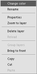
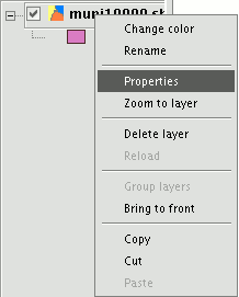
You can access the active layer's properties from its contextual menu (right click on the layer).
Capa vectorial
Cambiar el color de una capa añadida
Go to the layer’s contextual menu and click on the “Change colour” option. A window opens in which you can select the colour you wish to view the layer with.
There are three ways to select the colour depending on the window tab you select.
Swatches
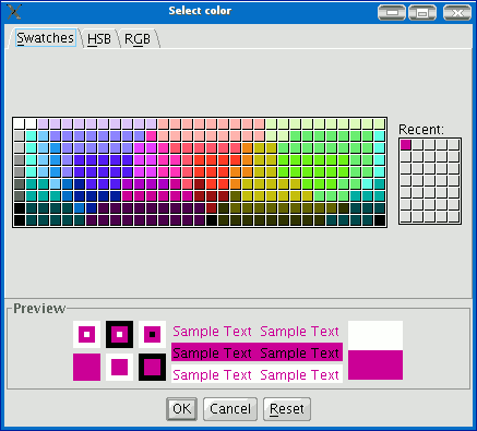
Selecting the colour from the “Swatches” tab is relatively easy. Place the mouse pointer over the desired colour on the palette and left click.
The colours you have used recently appear in the "Recent” palette.
HSB
A colour can be defined by its hue, brightness and saturation values. Any colour can be identified by values of these three variables. Black is obtained when there is an absence of light. Grey is obtained when the saturation is low (high light interference or mixture). White is the brightest colour of the greys (maximum frequency of different length waves).
This colour representation model is called HSB (Hue, Saturation, Brightness).
gvSIG has a colour selection window based on the HSB and RGB system which allows colour to be selected via HSB attributes and also obtain RGB values to reproduce them on the screen.
The following table shows the Hue variations which are represented on the horizontal axis of the square. The Saturation variations are represented on the vertical axis and the Brightness variations are shown on the side bar.
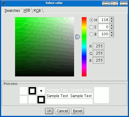
You can set one of the colour values by clicking on the corresponding check box. Click on the square area to define the values for the other 2 parameters. Slide the horizontal bar to set the value for the parameter marked with the check box.
When you have defined the colour you require, click on “Ok”.
RGB
RGB colour uses an additive model, in which the primary colours (red, green and blue) are combined to make other colours.
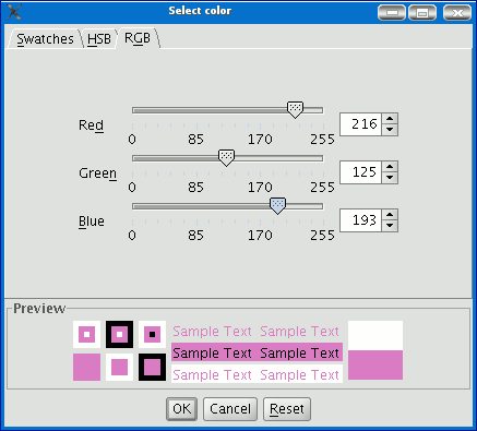
In this case, each primary colour is coded with a byte, so that each value is in a natural numbers [0, 255] interval. Thus, the RGB combination for black is R=0, G=0, B=0 and R=255, G=255, B=255 for white.
Cambiar el nombre a una capa añadida
If you wish to rename the selected layer, right click on the layer and go to the "Rename" option.
A new window appears:
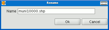
Write the new name in the text field and click on “Ok”.
N.B.: When you do this, the layer name changes in the ToC, but the file name is not changed.
Propiedades
Introducción
Right click on the selected layer in the ToC to access the properties window.

When you click on the “Properties” option, a new dialogue box opens. This can be used to edit some properties.
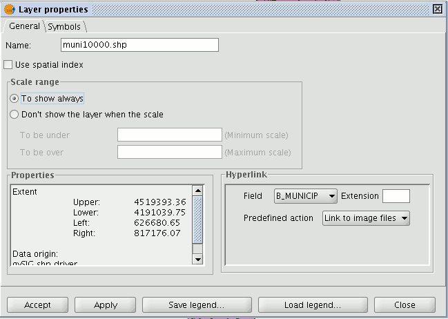
The layer name can be changed by writing the new name in the text field in the “General” tab.
Usar índice espacial
If you mark the “Use spatial index” check box, a spatial index will be created which makes the layer loaded in the view appear more quickly. This is because the view is loaded using this index.
If there are write permissions, a .qix file is created with the same name as the layer it is associated with in the layer’s original directory. If there are no write permissions, the file will be created in the user’s temporary file directory.
Rango de escalas
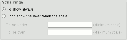
A viewing scale range (maximum and minimum) can be set in the properties window.
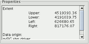
Resumen de las propiedades de las capa y su ruta de localización
The file extension and path are shown in the actual properties section.
Crear un hiperenlace en una capa
A link can be set up between a text, html or image file and a layer element in the properties window.
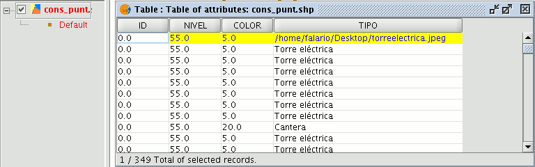
To provide a better idea of how the tool works, let us look at the following example. The aim is to link the image torreelectrica.jpg to a specific element:
Activate the view in the ToC.
Change the layer into editing mode (“Layer” menu then “Start edition”).
Open the table of attributes and edit the record you wish to create the link to. Write the path of the file you wish to link without its extension. Press “Enter” to save the modification made in the table.
Go to the “Hyperlink” table in the layer properties window and select the field the record is located in which will be used to create the hyperlink. Write the extension of the file you wish to link and whether it is an image file (gif, jpg, png) or a text file (at present gvSIG can only link plain text files (txt, rtf...). Html files can also be linked. In this case, write html in the “Extension” text box and select “Link to text files”.
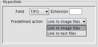
When all the requirements have been selected, click on “Apply” and then on “Ok”.
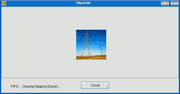
Then go the view tool bar and click on the hyperlink button.

Select the view element that corresponds to the record which has the associated link and place the cursor over it. Click on the element. A window appears with the linked file.
Editor de leyendas
Introducción
This tool can be used to carry out theme mapping relatively easily.
To symbolise or represent the element data or variables in a layer, you can choose the most suitable colour, pattern, etc. for each one.
Go to the “Properties” menu (right click on the layer) to edit the legend symbol properties.
A new window appears. Click on the “Symbols” tab.

Use this tab to define the legend type you wish to use to represent the layer data more specifically.
You can choose between the following:
Unique symbols: This is gvSIG’s default legend type and represents all the elements of a layer using the same symbol. It is useful if you need to show the location of a layer over and above any of its other attributes.
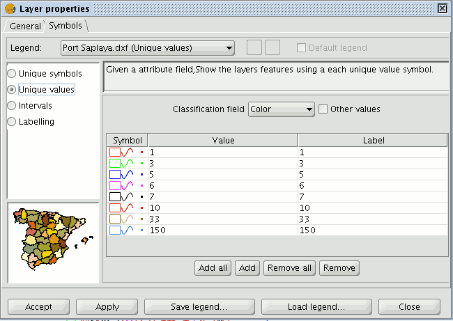
Unique values: Each record can be represented by a unique symbol according to the value it has in a particular field in the table of attributes. It is the most effective method to show categorical data, such as towns, types of land, etc.
Intervals: This type of legend represents the layer elements using a range of colours. The intervals or graduated colours are mainly used to represent numerical data which increase progressively or have a range of values, such as population, temperature, etc.
Labelling: Texts or labels can be automatically added to the view according to the values each element has in a particular field in its table of attributes.
The options shown in the symbols menu vary according to the type of layer (point, line or polygon layer).
The options available for a polygon layer, which has the most configuration tools, are shown below.
A legend can be saved or loaded (recovered) at any time.
Símbolo único
The following symbol configuration options are available:
Fill: Allows the fill colour to be selected.
Fill type: Allows the fill pattern to be selected.
Line: Allows the line colour to be selected.
Line style: Allows the style of the line to be selected.
Synchronising line and fill colours.
Line width: Allows the width of the line to be defined.
Transparency: Gives the elements a degree of transparency so that polygon layers can be superimposed and yet still viewed.
In point-type shape layers you can use the “Unique symbol” option in the “Symbols” tab to define the symbol type, the colour and point size you wish this layer to be displayed with.
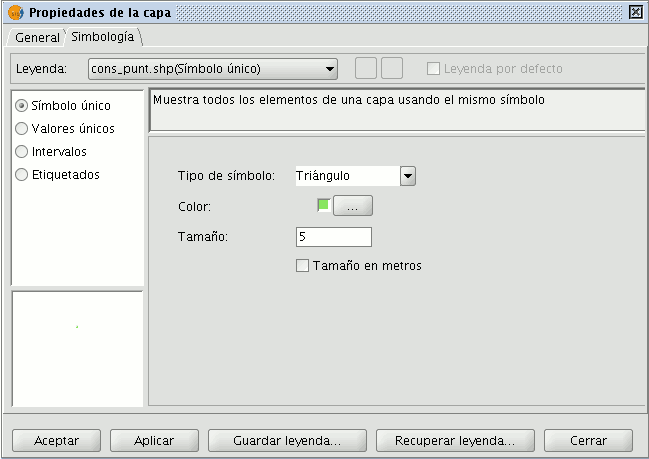
· Click on the “Symbol type” pull-down menu and select the symbol you wish the layer to be displayed with. Select the colour and set the size of the symbol you have chosen.
Click on “Apply” to see a preview of the set configuration.
Click on “Ok” if you wish to make this configuration permanent.
Click on the “Symbol type” pull-down menu and select the symbol you wish the layer to be displayed with. Select the colour and set the size of the symbol you have chosen.
Click on “Apply” to see a preview of the set configuration.
Click on “Ok” if you wish to make this configuration permanent.
Valores únicos
The following symbol configuration options are available:
Classification field: A pull-down menu appears in which you can select the layer’s table of attributes’ field which contains the data to be sorted.
Add all/Add: Once you have selected the “Classification field”, click on the “Add all” button to see all the different values. These values have all been assigned a different symbol (colour). Click on these symbols to modify them. By default, the label (the name which appears in the legend) is similar to the value it has in the field. You can include new values to the list by pressing the “Add” button.
Remove all/Remove: This allows all (Remove all) or some (Remove) of the elements in the legend to be removed.
Labels: Left click on any of the “Label” “cells” to modify the name they will have in the legend.
Intervalos
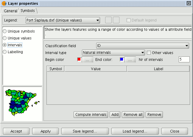
Classification field: A pull-down menu appears in which you can select the layer’s table of attributes’ field, which contains the data to be sorted. The field must be numerical because this is a gradual classification (by ranges of values).
Number of Intervals: This must indicate the number of ranges or intervals that define its classification.
Start colour and End colour: Select the colours to be graduated. The start colour is for the lowest values and the end colour is for the highest values.
Computing intervals: When you have defined the previous options, click on the “Compute intervals” button to see the legend’s end result. The symbols and the labels which appear by default can be modified by clicking on them, as in the previous cases.
Add: New ranges can be added to the computed intervals.
Remove all / Remove: This allows all (Remove all) or some (Remove) of the elements in the legend to be removed.
- Type of intervals: From gvSIG version 0.4 onwards, you can specify the interval type you wish to divide the information into in order to represent it. You can choose between the following options:
- Equal intervals: The number of intervals are specified and the sample is divided into this number of equal intervals.
- Natural intervals: The number of intervals is specified and the sample is divided into this number of intervals according to the Jenk method of optimising the natural breaks for the intervals.
- Quantile intervals: The number of intervals is specified and the sample is divided into this number of intervals but the values are grouped together according to their order number.
Etiquetado
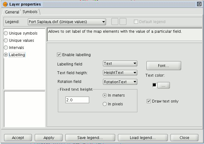
Enable labelling: Activate the check box to make the labelling visible in the view.
Labelling field: This is a pull-down menu which allows you to choose the layer’s table of attributes’ field, which contains the values to be shown as labels.
Text height field: This allows you to choose the layer’s table of attributes field which contains the values to be used for the label height.
Text rotation field: This allows you to choose the table of attributes field which indicates the label rotation angle.
Text colour: Allows the text colour to be selected.
Font: Allows the type of font to be selected.
Constant text height: Select the units (metres or pixels) and the text size. If you select “pixels”, the apparent text size will remain constant, even if you change the viewing scale; if you select “metres”, the text height on the display will vary according to the scale you are working in but will remain constant in geographic units.
Capa raster
Propiedades del raster
Right click on a raster layer and select the "Raster properties" option. This opens a menu in which we can carry out various operations on the raster layer.
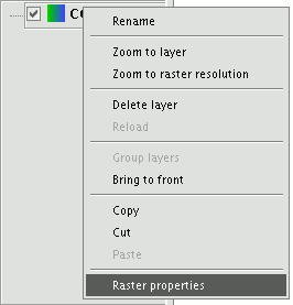
This menu is divided into five tabs:
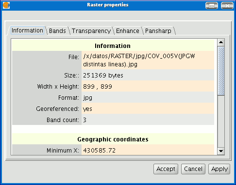
Information: Provides general information about the raster layer, the file path, the number of bands, the pixel dimensions, the file format, the data type and the geographic coordinates of the corners.
Bands: Provides tools to change the mode in which each image band is viewed. Transparency: Provides tools to change the transparency levels that can be applied to a raster layer.
Enhance: Provides a tool to enhance the raster layer. Pansharpening: Provides a tool to increase the satellite image resolution if the panchromatic band for these images is available.
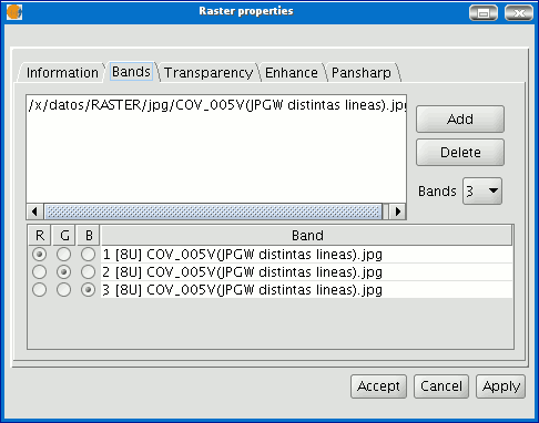
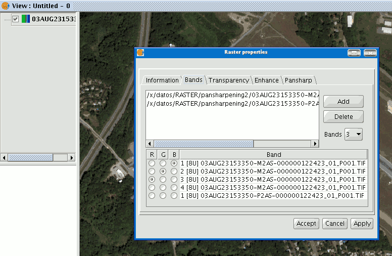
In the “Bands” tab you can make compositions using the different bands in a raster image. You can also add more bands from other files. This is useful when working with Landsat-type images, in which each band is delivered in a different file.
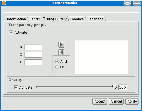
In addition to the “Transparency” option in gvSIg version 0.3, which is now called “opacity”, and which indicates the "occlusion” percentage of this layer over the previous ones, there is now a transparency option which allows the indicated colour groups (RGB) to be completely transparent. This is very useful to eliminate visual artefacts as a result of missing data in orthophotos or satellite images and to remove borders in an image mosaic.
To access the options, click on the corresponding “Activate” check boxes.
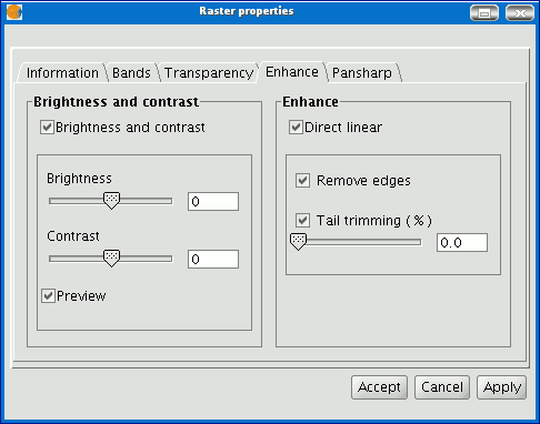
The “Enhance” tab can be used to modify the image brightness, contrast and enhancement. This last option is essential to be able to view 16-bits per band images correctly.
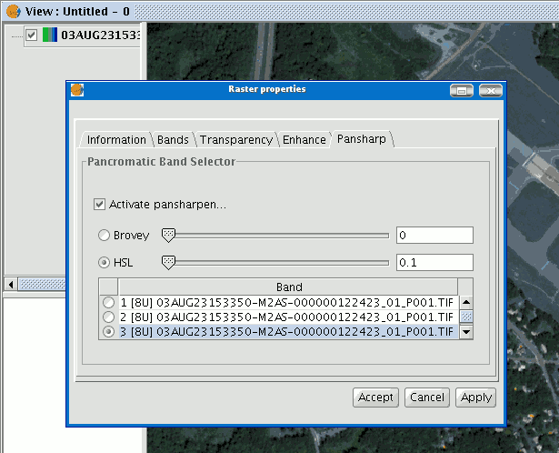
The “Pansharpening” tab can be used to increase the resolution of satellite images if the panchromatic band for these images is available. N.B.: If the image bands are in different files, they must be added to the layer using the “Bands” tab.
Use the “Bands” tab to find the best band combination for the view. In this section, you can load the image which corresponds to the panchromatic band but you must not select it to be visualised.
When the bands have been loaded, you can carry out the pansharpening. Go to the “Pansharpening” tab and activate it by clicking on the “Activate Pansharpening” check box. Select the panchromatic band with which the pansharpening is to be carried out from the band list. Finally, select an algorithm to be applied. There are two methods available, “Brovey” and “HSL”. Both of them have a slide bar control to carry out adjustments.
In “Brovey” the general brightness of the resulting image is increased or decreased.
In “HSL” the coefficient which is added to the brightness taken from the pansharpening band varies before it is replaced in the output image. This coefficient can vary between 0.15 and 0.5. When modified, the obtained result also influences the output image’s general brightness. If you click on the "Apply" or “Ok" buttons, the pansharpening will be applied on the image in the view, thus increasing the image resolution.